In [10]:
import numpy
import matplotlib.pyplot as plt
%matplotlib inline
In [11]:
I = numpy.eye(2)
Kc = 1

def G(s):
    return numpy.matrix([[3/(3*s + 1), 1/(s + 1)],
                         [1/(s+1), 3/(4*s + 1)]])

def K(s):
    return Kc*I

def L(s):
    return G(s)*K(s)

def sigmas(G):
    u, s, v = numpy.linalg.svd(G)
    return s

def RGA(G):
    return numpy.asarray(G)*numpy.asarray(G.I).T

def RGAnum(G):
    return numpy.abs(RGA(G) - I).sum()
In [23]:
omegas = numpy.logspace(-2, 2, 1000)
In [17]:
dets = []
OLsigmas = []
Tsigmas = []
RGAnums = []

for omega in omegass:
    s = 1j*w
    T = L(s)*(I + L(s)).I # Closed loop TF

    OLsigmas.append(sigmas(G(s)))
    Tsigmas.append(sigmas(T))
    RGAnums.append(RGAnum(G(s)))
    dets.append(numpy.linalg.det(L(s) + I))
dets = numpy.array(dets)
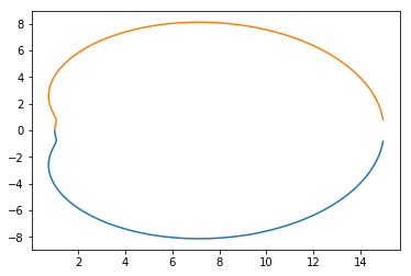
Multivariable Nyquist plot
In [5]:
plt.plot(dets.real, dets.imag, dets.real, -dets.imag)
Out[5]:
[<matplotlib.lines.Line2D at 0x11a44c898>,
 <matplotlib.lines.Line2D at 0x11a44ca20>]
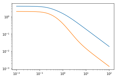
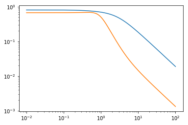
Singular values over frequency
In [6]:
plt.loglog(ws, numpy.array(OLsigmas))
Out[6]:
[<matplotlib.lines.Line2D at 0x11a53e470>,
 <matplotlib.lines.Line2D at 0x11a552550>]
In [7]:
allsigmas = numpy.array(OLsigmas)
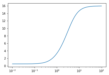
conditionnumber = allsigmas[:, 0]/allsigmas[:, 1]
plt.semilogx(ws, conditionnumber)
Out[7]:
[<matplotlib.lines.Line2D at 0x11af367f0>]
In [8]:
plt.loglog(ws, numpy.array(Tsigmas))
Out[8]:
[<matplotlib.lines.Line2D at 0x11b1539b0>,
 <matplotlib.lines.Line2D at 0x11b0e4f60>]
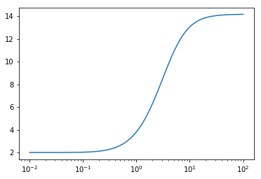
In [9]:
plt.semilogx(ws, RGAnums)
Out[9]:
[<matplotlib.lines.Line2D at 0x11b1ca588>]